Time-Series Forecasting at Scale
As of 2026-10-10
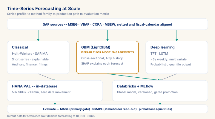
SAP demand and revenue forecasting fails less on model choice than on data hygiene: unnetted goods-issue reversals and fiscal-calendar drift alone can move a MASE score enough to flip a go/no-go on productionisation. For 90% of engagements the defensible sequence is a classical per-SKU baseline, then a single global LightGBM model with lag features -- the approach that won the M5 Walmart competition and now dominates SAP retail and distribution forecasting -- promoted to production only if it beats the baseline by more than 10% MASE on a holdout set. Where the client already runs HANA Cloud, PAL forecasts 50,000 SKU-series in under ten minutes without moving data; where complexity or volume outgrows PAL, Databricks with MLflow-gated promotion is the production path. Senior data scientists who can carry this decision end-to-end, SAP table-level data cleaning included, command EMEA day rates of 900-1,200 EUR in supply chain and 1,100-1,400 EUR in financial services.
What you will learn
- Select among classical statistical methods (Holt-Winters, ARIMA/SARIMA), gradient-boosted tree approaches (LightGBM, XGBoost), and deep-learning models (LSTM, TFT) based on dataset size, interpretability requirements, and operational complexity
- Operationalise time-series forecasting on SAP data using hana-ml/PAL, SAC Predictive Planning, and Databricks AutoML or MLflow
- Evaluate a forecast with appropriate metrics (MASE, SMAPE, pinball loss for quantile) and detect common failure modes specific to SAP data patterns
- Frame the business value, interpretability trade-offs, and infrastructure costs in client workshops and rate negotiations
Why SAP Time-Series Data Is Harder Than Benchmark Datasets
Most public time-series benchmarks (M4, M5, Kaggle demand forecasting competitions) use clean, regularly-spaced, complete series. SAP transactional data is none of these. Understanding this gap is the first practical skill for a consultant building forecasting solutions on SAP.
Irregular series -- SAP demand data (MBEW stock values, VBAP sales order quantities, COPA line items) is event-driven: a record exists when a transaction occurs, not at every calendar point. A material that sells three times a week in busy periods may go four weeks with zero transactions in slow seasons. Naively treating zero-transaction periods as missing data and interpolating introduces phantom demand; treating them as structural zeros and excluding them breaks seasonality estimation. The right approach is explicit intermittent demand modelling (Croston's method or its Syntetos-Boylan variant for slow-moving SKUs, ensemble with a standard model for regularly-selling items).
Prerequisites
- Intermediate hands-on experience on SAP analytics projects
- Review core concepts first: C087, C083, C069
Outcomes
- Work through a realistic scenario: A DACH industrial equipment manufacturer with 30,000 active materials across five plants is replacing spreadsheet-based demand planning ahead of a fiscal-year cutover.
- Recognize and avoid the anti-pattern: Training on raw MSEG postings without netting reversals — The model learns accounting artifacts (movement-type reversal pairs) as demand signal.
- Apply the module's core decision: Model family selection — choose Classical (Holt-Winters/SARIMA) below ~2 years of history or when auditors need explainable parameters.
- Track mastery with the KPI: Forecast accuracy (MASE) (target: MASE < 1.0 against the naive baseline on a 6-month holdout; red flag: MASE >= 1.0 -- the model loses to a random-walk forecast; do not promote).
Full module available to members. The full module adds: the decision framework · the end-to-end scenario walkthrough · the KPI scorecard · the anti-patterns · the code blocks · the knowledge check · the diagrams.